Dimensionality Reduction & Matrix Factorization I
Summary of Dimensionality Reduction & Matrix Factorization
Dimensionality Reduction & Matrix Factorization
차원 축소 Dimensionality Reduction 은 단순히 데이터를 줄이는 것이 아니라, hidden correlations 나 topics 를 발견하고 해석가능한 형태로 가공하는 강력한 도구이다. PCA/SVD 와 같은 Linear Method 부터, t-SNE/Autoencoder와 같은 non-linear method까지, 데이터의 특성과 목적에 맞는 모델선택이 중요하다.
Introduction: Unsupervised Learning and Dimension Reduction
Unsupervised Learning은 데이터 내부에 숨겨진 구조(latent structure) 를 찾는 과정으로 ,데이터 포인트 \(x\) 를 모델링하는 \(p(x)\) 의 관점에서 이해할 수 있다.
Motivation of Dim Reduction
- Curse of Dimensionality : 차원이 높아질수록 밀도를 규명하기 위해 기하급수적으로 많은 데이터가 필요하다.
- Computational Efficiency : 거리함수 계산복잡도를 낮추고 메모리를 절약한다.
- Visualization : 고차원데이터는 시각화하기 어렵지만, 데이터가 대개 저차원 매니폴드(**low-dim. manifold)에 내장되어 있다는 점을 이용해 가시화할 수 있다.
Linear Transformations
원본 데이터 \(X\) 를 직교변환행렬 \(F\) 를 통해 새로운 좌표계 \(X' = X \cdot F\)로 변환한다. 이때 평균 벡터를 \(\bar{x}\) 라고 하면, 변환된 공간에서의 평균은
\[\bar{x}' = \bar{x}\cdot F\]이며, 공분산 행렬은
\[\Sigma_{x'} = F^{T}\cdot \Sigma_{x}\cdot F\]Principal Component Analysis (PCA)
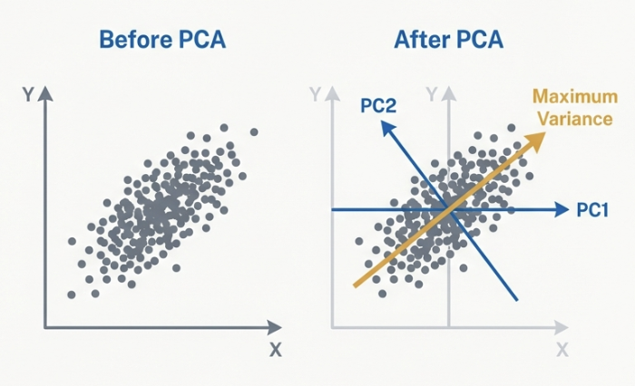
PCA 의 목적은 새로운 차원들 사이의 상관관계가 0이 되도록 좌표계를 변환해, Variance가 낮은 차원을 무시함으로써 데이터를 압축하는 것이다.
Given
- \(N \ d-\) dimensional data points: \(\{ x_i \}^N_{i=1}, x_i \in \mathbb{R}^d \ \forall i \in \{1, ..., N\}\)
그럼 우리는 \(X \in \mathbb{R}^{N \times d}\) 를 다음과 같이 나타낼 수 있다.
\[X = \begin{bmatrix} x_{11} & \cdots & x_{1d} \\ \vdots & \ddots & \vdots \\ x_{N1} & \cdots & x_{Nd} \end{bmatrix}\]\(\rightarrow\) Row \(x_i = \{ x_{i1}, ..., x_{id} \} \in \mathbb{R}^d\) 는 \(i\)-th point 를 뜻하며, column \(X_{:,j}\) 는 \(j\)-th dimension 의 모든 값을 포함하는 벡터를 뜻한다.
What this means in practice:
The covariance matrix of the transformed data becomes a diagonal matrix. All off-diagonal elements (covariances between different dimensions) are zero.
The new axes, called Principal Components, are ordered by the amount of variance they capture from the original data. The first principal component is the direction of maximum variance.
Method
1. Center the data : 평균 \(\bar{x} = \frac{1}{N} X^T \mathbb{1}_N\)을 구해서 데이터에서 뺀다.
\[\tilde{x}_{i} = x_i - \bar{x}\]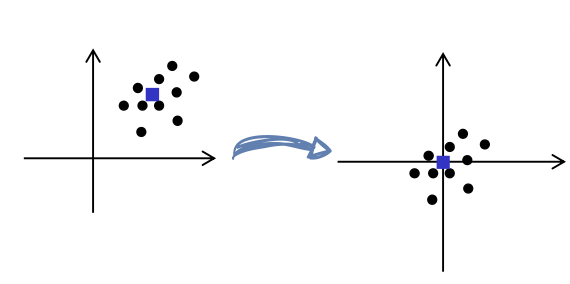
Statistics
Zero order statistic : number of points \(N\)
First order statistic : the mean of the \(N\) points, the vector \(\bar{x} \in \mathbb{R}^d\) : \(\bar{x} = \begin{bmatrix} \bar{x}_1 \\ \vdots \\ \bar{x}_d \end{bmatrix} = \frac{1}{N} \cdot X^T \cdot \mathbb{1}_N\)
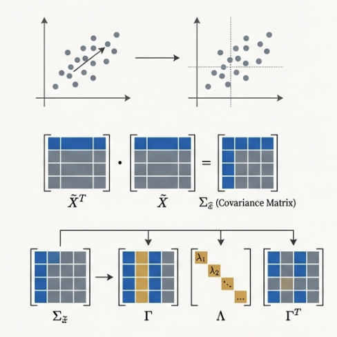
2. Compute Covariance Matrix : Covariance \(S\) (or \(Cov(\tilde{X}_j)\)) 를 계산한다.
\[S = \frac{1}{N} \sum^N_{n=1} (x_n - \bar{x})(x_n - \bar{x})^T\]Determine the Principal Components
Determine the variance \(Var(\tilde{X}_j)\) for each dimension \(j \in \{1, ..., d \}\)
Determine the covariance \(Cov(\tilde{X}_{j1}, \tilde{X}_{j2})\) between dimensions \(j_1\) and \(j_2, \ \forall j_1 \neq j_2 \in \{ 1, ... , d \}\)
Statistics
- Second order statistic : Variance and Covariance
The variance within the \(j\)-th dimension in $X$ is:
\[Var(X_j) = \frac{1}{N} \sum^N_{i=1} (x_{ij} - \bar{x}_j)^2 = \frac{1}{N} \cdot X^T_j X_j - {\bar{x}_j}^2\]The covariance between dimension $j_1$ and $j_2$ is:
\[Cov(X_{j1}, X_{j2}) = \frac{1}{N} \sum^N_{i=1} (x_{i j_1} - \bar{x}_{j_1}) = \frac{1}{N} \cdot X^T_{j_1} X_{j_2} - \bar{x}_{j_1} \bar{x}_{j_2}\]For the set of points contained in \(X\) the corresponding covariance matrix is defined as:
\[\Sigma_{X} = \begin{bmatrix} Var(X_1) & Cov(X_1, X_2) & \cdots & Cov(X_1, X_d) \\ Cov(X_2, X_1) & Var(X_2) & \cdots & Cov(X_2, X_d) \\ \vdots & \vdots & \ddots & \vdots \\ Cov(X_d, X_1) & Cov(X_d, X_2) & \cdots & Var(X_d) \end{bmatrix} = \frac{1}{N} X^{T} X - \bar{x}\bar{x}^{T}\]
3. Eigendecomposition : 공분산 행렬을 다음과 같이 분해한다.
\[\Sigma_{\tilde{X}} = \Gamma \cdot \Lambda \cdot \Gamma^T\]| Symbol | Description | |
|---|---|---|
| \(\Gamma\) | Eigenvectors Matrix 이고, 이들이 곧 Principal components 이다 | |
| \(\Lambda\) | Eigenvalues ($$\lambda | i$$)를 대각성분으로 가지며, 이는 새로운 차원에서의 분산을 의미한다 |
The result
Dimensionality Reduction : 고유값이 큰 순서대로 \(k\) 개의 Eigenvector 만 유지해서 \(Y_{\text{reduced}} = \tilde{X} \cdot \Gamma_{\text{truncated}}\) 를 얻는다. 보통 전체 Variance 90% 이상을 설명할 수 있ㄴ슨 \(k\) 를 선택한다.
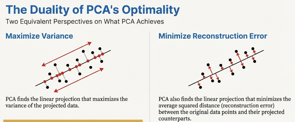
Variance : 분산을 최대화하는 방향을 찾는 것 (=Induction proof 과정)은 결과적으로 reconstruction error 를 최소화하는 것과 동일하다.
Dimensionality Reduction with PCA
Approach
- The coordinates with low variance (hence low \(\lambda_i\)) can be ignored
- W.l.o.g. let us assume \(\lambda_1 \ge \lambda_2 \ge \cdots \ge \lambda_d\)
Truncation of \(\Gamma\)
- Keep only the first \(k\) columns (eigenvectors) of \(\Gamma\) corresponding to the largest \(k\) eigenvalues \(\lambda_1,\ldots,\lambda_k\).
- Denote \(\Gamma_k = [\gamma_1,\ldots,\gamma_k] \in \mathbb{R}^{d\times k}\), then the reduced representation is \(Y = \tilde{X}\Gamma_k\).
How to pick k?
- Frequently used: 90% rule (explained variance ratio).
- Choose the smallest \(k\) such that \(\frac{\sum_{i=1}^{k}\lambda_i}{\sum_{i=1}^{d}\lambda_i} \ge 0.9.\)
Result
- The modified points (transformed and truncated) retain most of the information of the original points while being low-dimensional.
Complexity
\(O(N \cdot d^2) + O(d^3) + O(N \cdot d \cdot k) = O(N \cdot d^2 + d^3)\) compute covariance matrix + eigenvalue decomposition + project data onto the k-dim space
PCA Summary
PCA finds the optimal transformation by deriving uncorrelated dimensions (Exploits Eigendecomposition)
Dimensionality reduction
- After transformation simply remove dimensions with lowest variance
- or use only the \(k\) largest eigenvectors for transformation
Limitations
Only captures linear relationships (Solution: Kernel PCA)
Singular Value Decomposition (SVD)
Idea
데이터는 low-dimensional manifold (embedded in higher dimensional space) 에 있는 경우가 잦다.
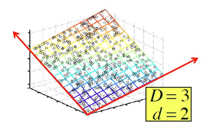
이 경우 이 매니폴드의 디멘셔을 어떻게 구할 수 있나? 여기서 rank 의 개념이 등장하는데, 결과적으로는 랭크가 곧 디멘션이다. 그리고 랭크는 coordinate 를 reduce 할 수 있다. 그럼 베스트 로우 랭크를 찾으면 되겠네! 하고 idea 가 시작된다.
Goal : Find the best low rank approximation
best = minimize the sum of reconstruction error
given matrix \(A \in \mathbb{R}^{n \times d}, \text{ find } B \in \mathbb{R}^{n \times d} \text{ with rank} (B) = k\) that minimizes \(\| A - B \|^2_F = \sum^N_{i=1} \sum^D_{j=1} (a_{ij} - b_{ij})^2\)
Singular Value Decomposition (SVD)
SVD 는 임의의 행렬 A 를 세 행렬의 곱으로 분해하는 것.
\[A = U \cdot \Sigma \cdot V^T\]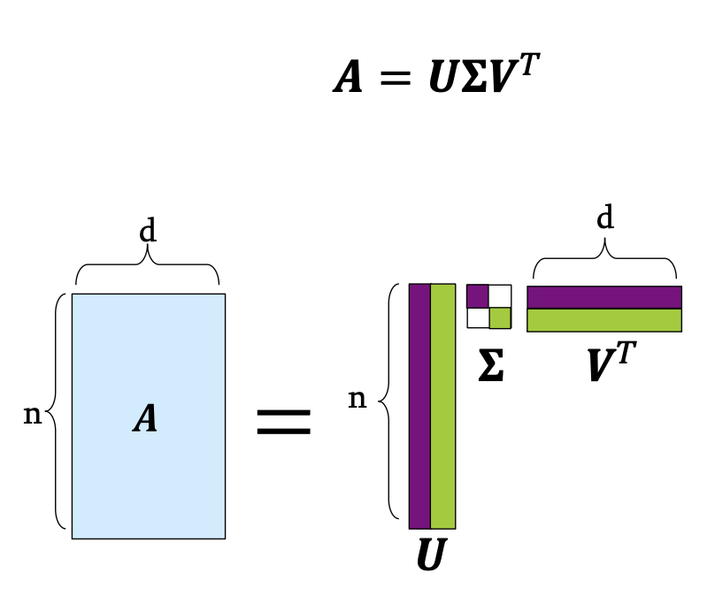
| Components | Description |
|---|---|
| \(U \in \mathbb{R}^{n \times r}\) | Left singular vectors, User-to-concept 유사도 |
| \(\Sigma \in \mathbb{R}^{r \times r}\) | Singular values(\(\sigma_i\)) 를 가진 대각행렬, concept’s strength |
| \(V \in \mathbb{R}^{d \times r}\) | Right singular vectors, Movie-to-concept 유사도 |
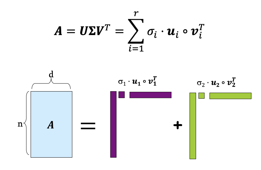
이렇게 세 행렬의 곱으로 나타내거나, 혹은 벡터의 합으로도 나타낼 수 있다.
Remark
The decomposition is (almost) unique!
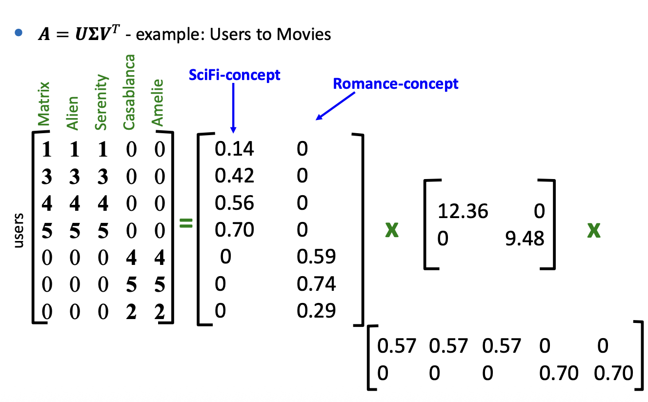
SVD - Example
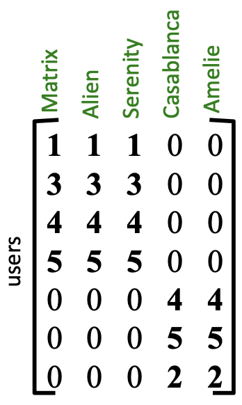
우리가 가진 데이터 매트릭스 \(A\) 는 다음 패턴을 따른다:
- 어떤 사용자는 특정 유형의 영화를 매우 선호한다.
- 어떤 영화들은 특정 genre에 속한다.
이것을 통해 어떤 사용자가 어떤 카테고리를 좋아하는지 추천시스템을 만들 수 있다. 우선 SVD 를 통해 우리의 매트릭스 \(A\) 를 분해하면 다음과 같다.
우리는 여기서
이런 관계를 알 수 있다.
- \(\Sigma\), Strength : 대각행렬로, singular values 가 들어 있다. 대각행렬 컴포넌트의 값이 클수록 그 패턴이 데이터에서 매우 지배적이다. 예를들어 \(\sigma_1 = 12.36\) 을 Sci-Fic 라고 하고, \(\sigma_2 = 9.48\)를 Romance 라고 부를 수 있다.
- \(U\), latent factors : 각 사용자가 우리가 발견한 latent concepts와 얼마나 일치하는지 보여준다.
- Sci-Fi, 첫번째 열의 값이 높은 사용자 1 - 4는 Sci-Fi 를 선호한다.
- Romance, 두번째 값이 높은 사용자 5-7 은 Romance 를 선호한다.
- \(V^T\), latent factors : 이 행렬은 영화를 동일한 latent concetps 에 매핍한다.
- Alien, Serenity 같은 영화들은 첫번째 행(Sci-Fi)에서 높은 값을 가진다.
- Casablanca, Amelie 는 두번째행 (Romance) 가 높다.
그런데 현실 데이터는 이렇게 깔끔하게 나뉜다기보다, 예를들어 어떤 사용자는 Sci-Fi AND Romance 를 모두 좋아할 수도 있다. 이렇게 실제 데이터에서는 \(U\) 와 \(V^T\) 가 0이 아닌 값들로 채워지는 blended 형태를 띈다.
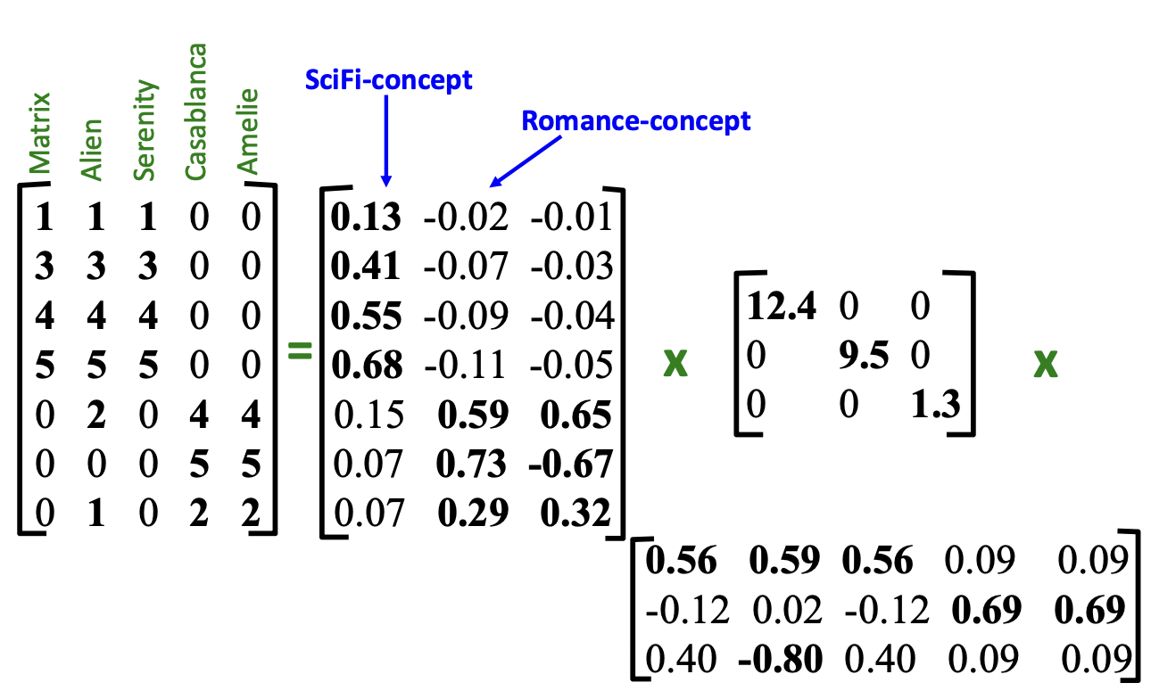
예를들어 사용자4는 Sci-Fi 와 0.68 만큼 강하게 연결되어 있으나, Romance 와는 -0.11 만큼 부정적으로 욘결되어 있다. 이처럼 SVD 는 사용자를 단순히 하나의 카테고리에 가두는 대신, 그 특성의 subtleties - 미묘한 차이 를 포착하는데 사용된다.
Low Rank Approximation
가장 작은 Eigenvalues 를 0으로 설정해서 matrix \(B\) 를 만들면, 이는 Frobenius norm \(\| A - B \|^2_F\) 을 최소화하는 최적읜 rank-k approximation 이 된다.
다음과 같은 행렬 \(A\) 를 우리는 \(B\) 로 similarization 할 수 있다.
\[A = \begin{bmatrix} 1.01 & 2.05 & 0.9 \\ -2.1 & -3.05 & 1.1 \\ 2.99 & 5.01 * 0.3 \end{bmatrix} \sim \begin{bmatrix} 1 & 2 & 1 \\ -2 & -3 & 1 \\ 3 & 5 * 0 \end{bmatrix} = B\]여기서 matrix \(B\) 는 rank(B) = 2 로, 행렬을 분석하기 더 쉬워진다. 이런식으로 쭉쭉 행렬을 0 과 비슷한것을 0으로 대체하면 차원이 줄어들고 rank 가 줄어들면 더 다루기 쉬워진다.
기하학적으로 해석을 해보자면 아래와 같다.
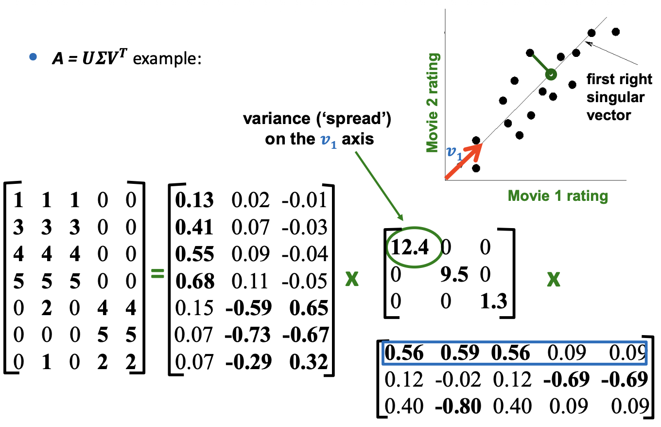
Best Low Rank Approximation
Let \(A = U \Sigma V^T (\sigma_1 \geq \sigma_2 \geq ..., \text{rank}(A)= r) \text{ and } B = U S V^T \text{ with } S\) being a diagonal \(r \times r\) matrix where
- \(s_i = \sigma_i \text{ for } i= 1, ..., k \text{ and } s_i = 0\) else
Then \(B\) is a best rank-k approximation to \(A\) regarding Frobenius norm. i.e., \(B\) is a solution to \(\min_{B} \| A - B \|_F \text{ where rank}(B) = k\)
앞서 언급한 복잡도는 다음과 같은데,
Complexity
\(O(N \cdot d^2) + O(d^3) + O(N \cdot d \cdot k) = O(N \cdot d^2 + d^3)\) compute covariance matrix + eigenvalue decomposition + project data onto the k-dim space
BUT:
- less work, if we just want singular values
- or if we want first k singular vectors
- or if the matrix is sparse
SVD vs. PCA
데이터 \(X\) 가 중앙에 정렬되있다고 했을때, \(X^T X = V \Sigma^2 V^T\) 가 성립해서 PCA’s Eigenvector 와 SVD’s right singular vectors(\(V\)) 가 일치하게 된다. 즉, SVD, PCA 는 linear dim reduction 관점에선 동일하다.
Matrix Factorization (MF) and Recommend System
실제 추천시스템에서는 데이터에 missing entries가 많아 클래시컬한 SVD 를 직접 적용하기 어렵다.
Latent Factor Models
\(r_{ui} \sim q_u \cdot p^T_i\) 를 통해 관측된 평점만으로 최적의 \(Q, P\) 를 찾는다.
최적화하느 기법은 OLS, SGD 등을 사용한다.
- Alternating Optimization : 한 변수를 고정하고 다른 변수를 Ordinary Least Squares (OLS) 로 최적화 하는 과정을 반복한다.
- Stochastic Gradient Descent (SGD) : 개별 평점에 대해 오차 \(e_{ui} = r_{ui} - q_u p^T_i\) 를 계산하고, 그래디언트 방향으로 파라미터를 업데이트한다.
Overfitting and Bias
데이터가 부족한 경우 모델이 노이즈를 학습하는 것으 막기 위해 Reularization 파라미터 \(\lambda_1, \lambda_2\) 를 도입할 수 있다.
\[\min_{P, Q} \sum (r_{ui} - q_u p^T_i)^ + \lambda_1 \sum \| q_u \|^2 + \lambda_2 \sum \| q_i \|^2\]또, 사용자별 관대함이나 영화의 전반적인 평점 수준을 반영하기 위해 유저 바이어스(\(b_u\)), item bias(\(b_i\)), global bias(\(b\)) 를 추가한다.
Advanced & Non-linear Methods
Non-Negative Matrix FActorization (NMF)
\(Q \geq 0, P \geq 0\) 제약을 두어 parts-based representation 과 더 ㄷ나은 해석력을 제공한다.
Neighbor Graph Methods
데이터의 전역 구조보다 local structure 를 보존하는데 집중한다.
- t-SNE이라는 기법으로, 고차원가 저차원 간 유사도 분포의 KL divergence를 최소화해 가시화에 탁월한 성능을 보인다.
Autoencoder
- Neural Network 를 사용한 nonlinear dim reduction methods
- Encoder (\(f_{enc}\)) 를 통해 저차원 Latent code(\(z\))로 압축하고, Decoder (\(f_{dec}\)) 를 통해 다시 복원하며 그 오차를 최소화한다.
- 만약 활성화 함수가 linear 라면, 이는 PCA 와도 수학적으로 동일한 결과를 낸다.