Feedback Linearization

Feedback Linearization

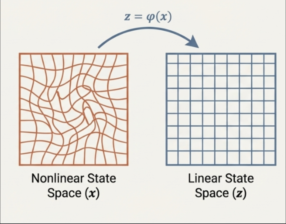
Feedback Linearization은 근사치에 의존하는 Taylor Series Lineaerization과 달리, Coordinate Transform과 non-linear feedback control input을 사용해 시스템을 비선형성을 없애고, 선형 시스템으로 변환하는 기법이다.

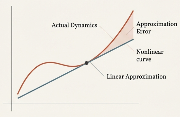
Taylor Series Linearization : An approximation valid only in a small neighborhood around an operating point.

Feedback Linearization : An exact system transformation, creating an equivalent linear system through a change of coordinates and feedback. Valid over a much larger region of the state space.

Lie Algebra

피드백 선형화를 이해하기 위해서는 , 미분 기하학적 도구인 Lie Derivative and Lie Bracket이 필요하다.

Lie Derivative

스칼라함수 \(h(x)\)를 벡터 필드 f(x)방향으로 미분하는 것을 의미한다.

\[L_f h := \nabla h \cdot f = \frac{\partial h}{\partial x } f(x)\]

이것을 여러번 미분하면 시리즈화 되는데, 형식은 다음 과 같다.

\[L^0_f h = h \text{ , } L^i_f h = L_f L^{i-1}_f h\]

Measures the rate of change of a function \(h\) along the vector field \(f\).

Lie Bracket

두 벡터 필드 \(f\)와 \(g\) 사이의 연산으로, 다음 처럼 정의된다.

\[[f, g] := L_f g - L_g f = \frac{\partial g}{\partial x} f - \frac{\partial f}{\partial x} g\]

Captures the non-commutativity of flows along vector fields \(f\) and \(g\).

마찬가지로 이것을 여러번 반복하면 시리즈화 되는데 이것을 Ad Operator 연산자를 사용한다.

Ad Operator

Lie Bracket을 반복적으로 적용하는 연산자로, 다음과같이 정의된다.

\[{ad}^0_f g = g \text{ , } {ad}^i_f g = [f, {ad}^{i-1}_f g]\]

Provides a compact notation fo repeated Lie Bracket

Relative Degree

The system \(\dot{x} = f(x) + g(x)\), \(y = h(x)\) has the relative degree \(r\) at point \(x^\circ\) if the following holds:

• For all \(x\) in the neighborhood of \(x^\circ\) and \(k < r - 1\):

$$ L_g L^k_f h(x) = 0 $$

• \[L_g L^{r-1}_f h(x^\circ) \neq 0\]

Input/Output (I/O) Linearization

시스템의 출력을 반복적으로 미분해서 입력 \(u\)가 직접 나타나게 함으로써 입출력 관계를 선형화하는 방법이다. 여기서 방금 언급한 Relative Degree가 사용된다.

Relative Degree \(r\)

출력 \(y\)를 \(r\)번 미분했을때, 비로소 입력 \(u\)가 식에 나타나는 경우, 이 시스템은 상대 차수 \(r\)를 가진다고 한다. 이 조건은 아까 언급한것과 같다.

다시말해 \(k > r - 1 \text{ 에 대해 } L_g L^k_f h(x) = 0 \text{ 이고, } L_g L^{r-1}_f(x^\circ) \neq 0\) 이어야한다.

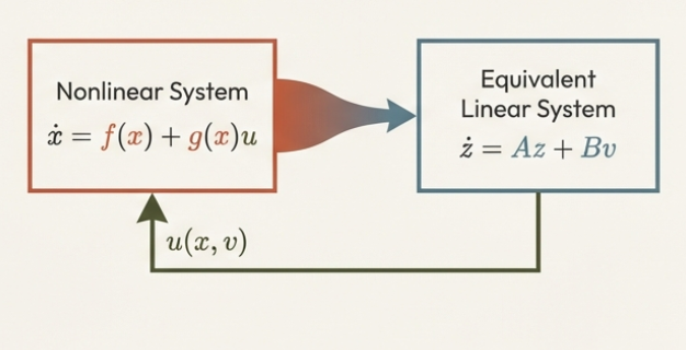
Linearizing Control Law - 선형화 제어 법칙

\(r\)번째 미분 식 \(y^{(r)} = L^r_f h(x) + L_g L^{r-1}_f h(x) u\)에서, 다음과 같은 Control Input, 제어입력을 설계한다.

\[u(x, v) = \frac{1}{L_g L^{r-1}_f h(x)} (v - L^r_f h(x))\]

이때 \(v\)는 새로운 가상의 입력이며, 최종적으로는 \(y^{(r)} = v^{**}\)라는 선형적인 integrator chain 관계를 얻게 된다.

이걸 왜하냐? 여러번 미분한 \(y^{(r)}= v\)를 새로운 문자로 사용할 수 있고, 그럼 여러차원의 미분의 계산이 매우 쉬워진다.

그럼 우리는 두 가지 케이스가 나온다.

• \(r=n\) : 이렇게 되면 풀랭크이고, \(n \times n\) 매트릭스의 formular가 온전하니까 Control Law를 사용하는데 전혀 문제가 없다.
• \(r < n\) : 이렇게 되면 어떻게 될까? 이때는 internal dynamics로 고려해야한다.

Internal Dynamics and Zero Dynamics - 내부 동역학

상대 차수 $r$이 시스템의 차수\(n\)보다 작은 경우\(r < n\), 출력에서 보이지 않는 \(n-r\) 차원의 Internal Dynamics 가 존재한다.

이때 Zero Dynamics라고 부르는데, 출력 \(y(t) \equiv 0\)으로 유지될 때의 내부 동역학 거동을의미하며, 이 시스템이 안정하기 위해서는 Zero Dynamics가 반드시 안정해야 한다.

Internal dynamics

I/O Linearization only transform \(r\) states. The remaining \(n - r\) states from the internal dynamics, which are not controlled by \(v\) or observed through \(y\).

If these internal dynamics are unstable, the entire system cam become unstable even if the input-output behavior appears perfectly controlled

This is the behavior of the internal dynamics when we force the output to be zero, i.e, \(y(t) \equiv 0\). The stability of the zero dynamics is a crucial test for the viability of the I/O linearization controller.

Full-State Linearization

시스템의 전체 상태 방정식을 선형 시스템으로 변환하는 기법이다. 특정 출력을 설계해서 상대 차수가 시스템 차수와 일치하게(\(r = n\)) 만드는 것과 같다.

Full-State Linearization

• Given : dynamics \(\dot{x} = f(x) + g(x)u\)
• Idea : directly design output \(y = \varphi_1 (x)\) with relative degree \(r = n\)
• Strategy : Solve the following PDEs, for some \(\mu^{*}(x) \neq 0\): \(\frac{\partial \varphi_1 (x)}{\partial x} \cdot \left[ g(x), \text{ad}_f g(x), ... , \text{ad}^{n-1}_f g(x) \right] = \left[0, ..., 0, \mu^{*}(x)\right]\)

\(\Rightarrow\) Full-state Linearization :

• State transformation

\[z = \varphi(x) := \left[ \varphi_1 (x), ..., L^{n-1}_f \varphi_1 (x) \right]^T\]

• Linearizing feedback

\[u(x) = \frac{1}{L_g L^{n-1}_f \varphi_1 (X)} \left( v - L^n_f \varphi_1 (x) \right)\]

Necessary and Sufficient Conditions - 필요충분조건

System \(\dot{x} = f(x) + g(x)\)가 Full-state Linearization이 가능하려면 다음 두 가지 조건을 만족해야 한다.

1. Reachability (가도달성) \(S(x)\) : Reachability Matrix 의 Rank 가 $n$ 이어야 한다.

\[\begin{aligned} & S(x) = \left[ g, \text{ad}_f g(x), ..., \text{ad}^{n-1}_f g(x) \right] \\ & \text{rank} \left( S(x) \right) = n \end{aligned}\]

2. Involutivity : 벡터 필드 집합 \(\left( g, \text{ad}_f g(x), ..., \text{ad}^{n-2}_f g(x) \right)\) 가 Involutive 해야한다.

즉, 이 집합 안의 벡터들끼리 Lie Bracket을 취한 결과가 다시 그 집합의 span 안에 있어야함

수식으로 표현하면 다음과 같다.

\[\begin{aligned} \mathcal{B} (x) &= \left\{ g(x), \text{ad}_f g(x), ... , \text{ad}^{n-2}_f g(x) \right\} \\ \left[ \text{ad}^i_f g, \text{ad}^j_f g \right] &\in \text{span}(\mathcal{B}) \text{ , for all } i, j \in \left\{ 0, ..., n - 2 \right\} \end{aligned}\]

State Transformation - 상태변환

• 새로운 좌표 $z = \phi(x)$를 착기 위해 다음의 PDE를 푼다.:

\[\frac{\partial \varphi_1}{\partial x} \left[ g, \text{ad}_f g, ..., \text{ad}^{n-2}_f g \right] = 0 \text{ and } \frac{\partial \phi_1}{\partial x}\text{ad}^{n-1}_f g \neq 0\]

-이를 통해 얻은 $z$ 좌표계에서는 시스템이 Controllable Canonical Form으로 표현된다.

Diffeomorphism - 미분 동상 사상

선형화 과정에서 사용하는 State Transformation $z = \phi(x)$ 가 유효하기 위한 조건이다.

• Local Diffeomorphism : \(\phi(x)\) 가 연속적으로 미분 가능하고, Jacobian Matrix \(\nabla \phi\) 가 \(x_0\) 에서 non-singular (=역행렬 존재) 해야 한다.

• Global Diffeomorphism : 모든 \(x\) 에서 Jacobian이 Regular(정칙)이고, \(x\) 가 무한대로 갈 때, \(\phi(x)\) 도 무한대로 가는 Proper 성질을 만족해야 한다.

Comparison: I/O vs. Full-State Linearization

I/O Linearization

우리가 관심 있는 특정 출력 \(y\) 를 선형화하는데 집중하지만, Internal Dynamics의 안정성으 따로 확인해야 하는 부담이 있다.

Full-State Linearization

시스템 전체를 선형화하므로 Internal Dynamics 문제가 발생하지 않지만, 이를 위한 출력 함수 \(\phi_1(x)\) 을 찾기 위해 복잡한 PDE를 풀어야 한다.