Support Vector Machines (SVM) and Kernels
Summary of SVM, Kernels
Support Vector Machines (SVM) and Kernels
Suppoer Vector Machines (SVM) - Hard Margin
SVM은 두 클래스를 분리하는 최적의 hyperplane을 찾는 linear binary classifier이다.
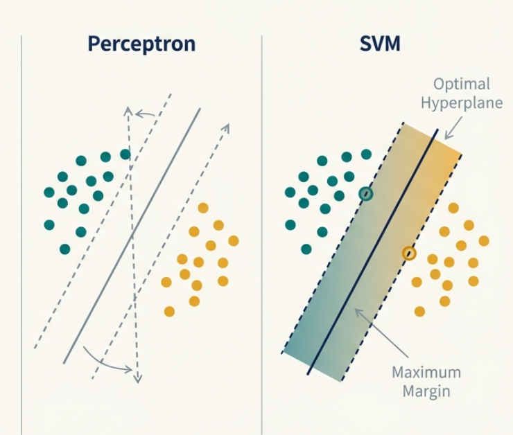
그럼 지금까지 본 Perceptron과 다른 SVM의 특징이 무엇일까?
공통점: Both are supervised methods that find a hyperplane &w^T x + b = 0& to separate two classes.
differences:
Perceptron Finds any separating hyperplane. Its solution can be arbitrary and depends on the starting point and data order
SVM Find the unique hyperplane that maximizes the margin. the distance to the nearest data points of any class
Maximum Margin Classifier
단순히 클래스를 분류하는 것을 넘어, 두 클래스 사이의 거리를 최대화하는 margin을 찾는 것이 목표이다. 이것은 새로운 샘플에 대해 더 나은 generalization 성능을 제공하기도 한다.
Decision Boundary
클래스 $h(x)$는 다음식에 의해 결정된다. \(h(x) = \text{sign}(w^T x + b)\)
Size of the Margin
두 클래스 평행 평면 사이의 거리인 margin은 다음처럼 정의된다.
\[m = \frac{2}{||w||} = \frac{2}{w^T w}\]| 왜냐하면 두 클래스에 대해 수직이기 때문. 우리는 이 margin $m$을 maximize하기 위해 무엇을 해야할까? 바로 $ | w | $를 최소화해야한다. 조금 더 쉽게 최소화하기 위해 우리는 이 최적화 문제를 다음 처럼 바꿀 수 있다. |
Primal Optimization Problems and its solution
\[\min_{w,b} \frac{1}{2} w^T w\]그런조건이 붙는다. 바로 Every data point must be on or outside the correct side of its margin boundary. 이를 수식으로 표현하면, :
\[\text{subject to } y_i(w^T x_i + b) - 1 \geq 0 \ i = 1,...,N\]Constrained optimization Problem
$ \text{Given} f_0 : \mathbb{R^d} \rightarrow \mathbb{R} \text{and} f_i : \mathbb{R^d} \rightarrow \mathbb{R}, $
$$ \text{minimize}_{\theta} \ f_0(\theta) $$ $$ \text{subject to} \ f_0(\theta) \geq 0, i = 1, ..., M $$ Feasibility A point $\theta \in \mathbb{R}^d$ is called feasible if and only if it satisfies the constraints of the optimization problem $ \text{i.e. } f_i(\theta) \leq 0, \text{ for all } i \in { 1, …., M}$
Minimum and minimizer We call the optimal values the minimum \(p^{*}\) and the point where the minimum is obtained the minimizer \(\theta^{*}$. Thus\)p^{} = f_0(\theta^{})$$
이 제약조건을 포함하기 위해 우리는 Lagrangian을 정의한다.
\[L(w, b, \alpha) = \frac{1}{2} w^T w - \sum^N_{i=1} \alpha_i [y_i(w^T w_i + b) - 1]\]그리고 Dual Problem 도 만들수 있는데, 이것은 $\alpha$에 대한 최적화 문제로 변환할때 사용한다.
Complementary slackness: Karush-Kuhn-Tucker (KKT)
이것은 SVM의 최적화 과정에서 Support Vectors를 정의하고 decision boundary를 확정 짓는 핵심적인 수학적 조건이다.
Strong duality가 성립할때, Primal 의 최적해 (\(\theta^{*}\))와 dual문제의 최적해 (\(\alpha^{*}\)) 사이에는 다음 관계가 성립한다.
\[\alpha^{*}_i f_i (\theta^{*}) = 0, \text{ for all } i = 1, ..., N\]여기서 $\alpha_i$는 Lagrange multiplier이고, $f_i(\theta)$는 Primal 문제의 제약조건이다. 이 식은 두 값 중 하나는 반드시 0이어야 함을 의미한다. 즉, $\alpha_i > 0$ 이면 \(f_i(\theta^{*})\) 이어야하고, 반대로 \(f_i(\theta^{*})\)이면, $\alpha_i$는 $0$이어야 한다.
Hard-margin SVM에서의 Constraint는
\[y_i (w^T x_i + b) - 1 \geq 0\]이다. 이를 Complementary slackness 식에 대입하면:
\[\alpha_i [y_i(w^T x_i + b) - 1] = 0\]이 조건에 따라 데이터 포인트는 두가지로 나뉜다.
- Case 1: $\alpha_i = 0 $
- 이 데이터 포인트는 weight vector $w$를 결정하는 식 $w = \sum \alpha_i y_i x_i$ 과 무관하다.
- 대부분의 데이터 포인트가 이 경우이고, 결과적으로 SVM has sparse solution
- Case 2: $\alpha_i < 0$
- Durch complementary slackness, gilt: $y_i (w^T x_i + b ) - 1 = 0$
- 즉, 이 포인트들은 정확히 margin위에 놓여 있는 데이터들이다.
- 이 포인트들만이 decision boundary 의 방향과 위치를 결정하고, 이를 Support Vectors라고 부른다.
Soft Margin Support Vector Machines
데이터가 노이즈에 있거나 선형적으로 분리되지 않는 경우에도 작동할 수 있게 설계된 모델이다. Hard-margin SVM 에서는 단 하나의 outlier만 있어도 Constraint를 만족하는 해를 찾지 못하거나, decision boundary가 크게 왜곡될 수도 있다. 그래서 이 constraint를 완화하기 위헤 slack variables(\(\xi_i\))를 도입한다.
Slack variables(\(\xi_i\))
각 샘플이 margin을 얼마나 위반했는지를 나타내는 거리이다. 각 training sample $x_i$ 에 대해 slack variable $\xi_i \geq 0$ 를 도입한다. 그럼 위반 정도에 따라 다음처럼 분류된다.
| Range | Classification | |
|---|---|---|
| 1 | $\xi_i = 0$ | 샘플이 margin위에 있거나 올바른 영역에 위치함 |
| 2 | $0 < \xi_i < 1 $ | 샘플이 margin 내부에 있지만, 여전히 올바른 클래스로 분류됨. |
| 3 | $\xi_i > 1 $ | 샘플이 결정경계를 넘어 잘못된 클래스로 분류됨 |
이것을 추가해 새로운 Primal optimization problem을 만든다.
여기서 #C#는 Penalty Parameter로, 위반에 대해 얼마나 엄격할지 결정한다. $C$가 매우 크면 ($C \rightarrow \inf $ Hard-margin SVM과 동일해지고, $C$가 작을 수록 더 큰 margin을 얻기 위해 더 많은 오분류를 허용한다.
Optimization problem with slack variables
Let \(x_i\) be the \(i\)th data point, \(i = 1, ..., N\), and \(y_i \in \{ -1, 1\}\) the class assigned to \(x_i\). Let \(C > 0\) be a constant. Then,
\[\min f_0 (w, b, \xi) = \frac{1}{2} w^T w + C \sum^N_{i=1} \xi_i\] \[\text{subject to } y_i(w^T x_i + b) - 1 + \xi_i \geq 0\] \[\xi_i \geq 0\]
Hard-margin SVM과 같이, 이를 Lagrangian과 함께 나타내면 다음과 같다.
1. Calculate Lagrangian:
\[L(w, b, \xi, \alpha, \mu) = \frac{1}{2} w^T w + C \sum^N_{i=1}\xi_i - \sum^N_{i=1} \alpha_i[y_i(w^T x+i + b) - 1 + \xi_i] - \sum^N_{i=1} \mu_i \xi_i\]2. Minimize \(L(w, b, \xi, \alpha, \mu)\) w.r.t. \(w, b\) and \(\xi\):
\[\nabla_w L(w, b, \xi, \alpha, \mu) = w - \sum_{i=1}^{N} \alpha_i y_i x_i \stackrel{!}{=} 0;\] \[\frac{\partial L}{\partial b} = \sum_{i=1}^{N} \alpha_i y_i \stackrel{!}{=} 0,\] \[\frac{\partial L}{\partial \xi_i} = C - \alpha_i - \mu_i \stackrel{!}{=} 0 \text{ for } i = 1, \dots, N\]From $\alpha_i = C - \mu_i$ and dual feasibility $\mu_i \ge 0, \alpha_i \ge 0$ we get
\[0 \le \alpha_i \le C.\]Dual Problem & Box Constraint
Soft-margin의 Dual formulation은 Hard-margin 과 거의 동일하지만, weight $\alpha_i$에 대해나 상한선이 추가 된다.
이떄 $ 0 \leq \alpha_i \leq C$ 를 Box constraint라고 하고, 이것은 특정 샘플이 decision boundary에 미치는 영향력을 $C$로 제한해서 outlier에 의한 폭주를 방지한다.
Complementary Slackness and Support Vectors
최적해에서 Complementary slackness조건에 따라 Support Vectors는 다음 특성을 보인다.
| Range | Slack | Classification | |
|---|---|---|---|
| 1 | $0 < \alpha_i < C$ | \(\xi_i = 0\) | 샘플은 정확히 margin 위에 놓여있다 |
| 2 | $\alpha_i = C$ | $\xi_i > 0$ | 샘플은 margin 을 위반한 상태로, 경계 안쪽이나 오분류 |
| 3 | $\alpha_i = 0$ | weight $w$ 계산에 기여하지 않고, margin 바깥 올바른 위치에 있다. |
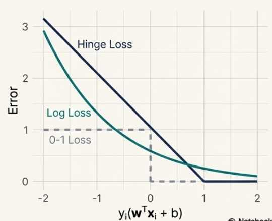
Hinge Loss Formulation
Soft-margin SVM은 제약조건 없는 최적화 문제로 재구성 할 수 있는데, 이를 hinge loss formulation이라고 한다. 식은 다음과 같다.
\[\min_{w,b} \frac{1}{2} w^T w + C \sum^N_{i=1} \text{max} \{0, 1 - y_i(w^T x_i + b)\}\]여기서 $ \text{max} {0, 1 - z }$를 Hinge loss 라고 부르며, 이것은 margin을 위반하는 포인트들에만 벌점을 부여하는 시스템이다. 이 방식은 gradient descent를 통해 직접 최적화가 가능하다는 장점이 있다.
Logistic Regression 과의 관계
Soft-margin SVM과 Logistic Regression은 구조적으로 매우 유사하다.
- common: 두 모델 모두 L2 regularization(\(\lambda w^T w\))를 공통적으로 사용한다.
- different: Loss function의 형태가 다르다.
| Model | Loss function | - |
|---|---|---|
| SVM | Hinge Loss | \(\min_{w,b} \frac{1}{2} w^T w + C \sum^N_{i=1} \text{max} \{0, 1 - y_i(w^T x_i + b)\}\) |
| Logistic Regression | Log Loss | \(ln(1 + exp^{-y(w^T x + b)})\) |
Kernels
데이터가 원래 공간엔서 선형 분리가 불가능할때, 고차원 feature space로 매핑해서 선형 분리를 시도하는 기법이다. 가장 큰 장점은 무한 차원의 basis function을 사용하는 것과 같은 효과를 낼 수 있다는 것(e.g., Gaussian kernel), 그리고 문자열이나 그래프 같은 비수치적 데이터의 유사도도 정의할 수 있다는 것이다.
Kernel Trick
Dual 수식에서 데이터가 항상 내적(\(x_i^T x_j\))의 형태로만 존재한다는 점을 이용한다. 명시적으로 고차원 매핑(\(\phi (x)\))을 계산하는 대신, 내적함수\(k(x_i, x_j) = \phi (x_i)^T \phi(x_j)\) 를 직접 이용한다.
이런 커널 트릭은 SVM 뿐만 아니라 다른 어떤 모델에서도 내적이 이용된다면, 사용할 수 있다.
Valid Kernel - Mercer’s Theorem
어떤 함수가 유효한 커널이 되려면, 임의의 데이터에대해 Kernel matrix(\(K\))가 1.symmetric하고 2.positive semi-definite해야 한다.
Mercer’s theorem
A kernel is valid if it gives rise to a symmetric, positive semidefinite kernel matrix \(K\) for any input data \(X\).
Kernel matrix (a.k.a Gram matrix) $K \in \mathbb{R}^{N \times N}$ is defined as
\[\mathbf{K} = \begin{pmatrix} k(\mathbf{x}_1, \mathbf{x}_1) & k(\mathbf{x}_1, \mathbf{x}_2) & \cdots & k(\mathbf{x}_1, \mathbf{x}_N) \\ k(\mathbf{x}_2, \mathbf{x}_1) & k(\mathbf{x}_2, \mathbf{x}_2) & \cdots & k(\mathbf{x}_2, \mathbf{x}_N) \\ \vdots & \vdots & \ddots & \vdots \\ k(\mathbf{x}_N, \mathbf{x}_1) & k(\mathbf{x}_N, \mathbf{x}_2) & \cdots & k(\mathbf{x}_N, \mathbf{x}_N) \end{pmatrix}\]
만약 non-valid kernel을 사용하면 어떻게 될까? 우리의 최적화문제도 non-convex가 되면서, 우리는 어떠한 최적해도 가질 수 없게 된다.
Kernel이 좋은 점이 또 하나 있는데, 상당히 많은 operatins가 유효하다는 것이다.
Let $k_1 : \mathcal{X} \times \mathcal{X} \to \mathbb{R}$ and $k_2 : \mathcal{X} \times \mathcal{X} \to \mathbb{R}$ be kernels, with $\mathcal{X} \subseteq \mathbb{R}^N$. Then the following functions $k$ are kernels as well:
- $k(\mathbf{x}_1, \mathbf{x}_2) = k_1(\mathbf{x}_1, \mathbf{x}_2) + k_2(\mathbf{x}_1, \mathbf{x}_2)$
- $k(\mathbf{x}_1, \mathbf{x}_2) = c \cdot k_1(\mathbf{x}_1, \mathbf{x}_2)$, with $c > 0$
- $k(\mathbf{x}_1, \mathbf{x}_2) = k_1(\mathbf{x}_1, \mathbf{x}_2) \cdot k_2(\mathbf{x}_1, \mathbf{x}_2)$
- $k(\mathbf{x}_1, \mathbf{x}_2) = k_3(\phi(\mathbf{x}_1), \phi(\mathbf{x}_2))$, with the kernel $k_3$ on $\mathcal{X}’ \subseteq \mathbb{R}^M$ and $\phi : \mathcal{X} \to \mathcal{X}’$
- $k(\mathbf{x}_1, \mathbf{x}_2) = \mathbf{x}_1^T \mathbf{A} \mathbf{x}_2$, with $\mathbf{A} \in \mathbb{R}^N \times \mathbb{R}^N$ symmetric and positive semidefinite
Examples of kernels
그렇다면 전형적인(?) 커널 양상을 알아보자.
| Kernel | Formula |
|---|---|
| Polynomial | $k(\mathbf{a}, \mathbf{b}) = (\mathbf{a}^T \mathbf{b})^p$ or $(\mathbf{a}^T \mathbf{b} + 1)^p$ |
| Gaussian (RBF) | $k(\mathbf{a}, \mathbf{b}) = \exp(-\frac{|\mathbf{a} - \mathbf{b}|^2}{2\sigma^2})$ |
| Sigmoid | $k(\mathbf{a}, \mathbf{b}) = \tanh(\kappa \mathbf{a}^T \mathbf{b} - \delta)$ for $\kappa, \delta > 0$ |
Sigmoid kernel은 정확히는 PSD는 아니지만, 잘 활용된다. 참고로 여기의 Sigmoid Kernel은 Sigmoid Function(from Linear behavior)와 다른 것임.
Summary
Dual function의 행렬 표현: Dual 함수는 $g(\alpha) = \frac{1}{2}\alpha^T Q\alpha + \alpha^T 1_N$으로 쓸 수 있으며, 여기서 $Q = -yy^T \odot XX^T$이다. $Q$가 negative semi-definite 하므로 이 최적화 문제는 concave하며, global maximum을 보장합.
LOOCV Error Bound: 전체 데이터셋에서 학습했을 때의 support vector 수를 $s$, 데이터 수를 $N$이라 할 때, Leave-one-out cross validation의 오차율 $\epsilon$은 $\epsilon \le \frac{s}{N}$의 관계를 만족한다. 이는 support vector가 아닌 데이터를 뺐을 때는 결정 경계가 변하지 않기 때문
Multiclass Classification: 표준 SVM은 binary classifier이므로, 여러 클래스를 처리하기 위해 One-vs-rest (한 클래스 대 나머지) 또는 One-vs-one (모든 쌍 조합) 전략을 사용.
<div class=”pdf-viewer-container” data-pdf=”/assets/img/posts/study-ml/ch9-svm.pdf” data-page=”13></div>